Geometric intuition of Matrix

Geometric Intuition of Matric

A matrix is first and foremost a mathematical form. Mathematics and geometry are deeply intertwined, so understanding matrices geometrically is quite interesting.
Work in many fields depends on matrices, so this article collects a few ways of understanding them as notes.

Matric

From the Vector Viewpoint

Consider the example matrix $\mathbf{X}\in \mathbb{R}^{2\times 3}$： $$\mathbf{X}= \begin{bmatrix} 1 & 2 & 3\\ 4 & 5 & 6 \end{bmatrix}$$

Row Vectors and Column Vectors

This is a matrix with 2 rows and 3 columns. If we focus on the row and column viewpoints respectively, it can be described as:

• Row viewpoint. This is a matrix composed of 2 row vectors $v$, where $\mathbf{v} \in \mathbb{R}^{1\times 3}$
• Column viewpoint. This is a matrix composed of 3 column vectors $v$, where $\mathbf{v} \in \mathbb{R}^{1\times 2}$

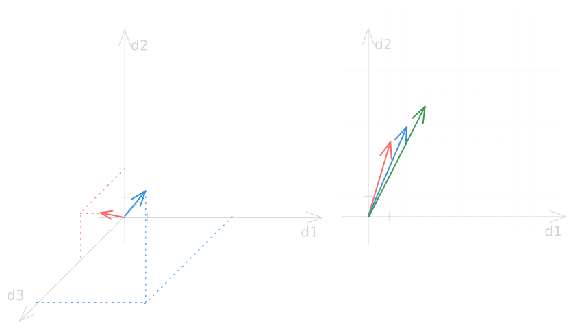
Under the row and column viewpoints, the matrix can be written as: $$\mathbf{X}_{\text{row}}= \begin{bmatrix} \color{#ff8383}1 & \color{#ff8383}2 & \color{#ff8383}3\\ \color{#56a2e8}4 & \color{#56a2e8}5 & \color{#56a2e8}6 \end{bmatrix} \qquad \mathbf{X}_{\text{col}}= \begin{bmatrix} {\color{#ff8383}1} & {\color{#56a2e8}2} & {\color{#39994b}3}\\ {\color{#ff8383}4} & {\color{#56a2e8}5} & {\color{#39994b}6} \end{bmatrix}$$

Geometric intuition for row and column vectors

One-Dimensional Matrix Vectors

Among them, a single-row or single-column matrix plays an even more special role. Taking a single-row matrix as an example, let $\mathbf{X}\in \mathbb{R}^{1\times 2}$.
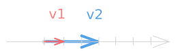
From the column viewpoint: $$\mathbf{X}= \begin{bmatrix} {\color{#ff8383}1} & {\color{#56a2e8}3} \end{bmatrix}$$

Its column-vector space is:

Geometric intuition for one-dimensional column vectors

This intuition will be used later in the geometric interpretation of the dot product of two vectors.

That is enough for the vector part for now.

From the Graph Viewpoint

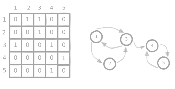
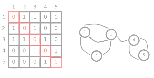
Matrices also have a geometric intuition in graph theory. For example: $$\mathbf{A}= \begin{bmatrix} 0 & 1 & 1 & 0 & 0 \\ 0 & 0 & 1 & 0 & 0 \\ 1 & 0 & 0 & 1 & 0 \\ 0 & 0 & 0 & 0 & 1 \\ 0 & 0 & 0 & 1 & 1 \end{bmatrix} \in \mathbb{R}^{5\times 5}$$

Directed Graphs

From the row viewpoint, it can be realized as 5 points in a graph space, with each row being a point in 5 dimensions.
For each point, dimension $n$ represents the relation between that point and the $n$-th point, which appears as an edge in graph space. Directed graph

If we extend the matrix entries from just 0 and 1 to more values, then the edges representing those relations can also encode weights: Directed weighted graph

Undirected Graphs

We can adjust the edge relationships by changing the matrix values, turning it into an undirected graph.

Undirected graph (notice the local symmetry)

Graph Connectivity

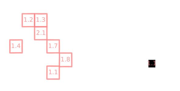
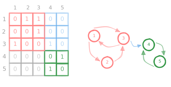
Now let us return to the original matrix and observe it from the perspective of connectivity. The whole graph can be divided into:

• strongly connected components (the red and green parts)
• the component-connecting region (the blue part)

Graph connectivity

Matrix Operations

Matrix Addition and Subtraction

If two matrices $\mathbf{A}\in \mathbb{R}^{n_1\times m_1}$ and $\mathbf{B}\in \mathbb{R}^{n_2\times m_2}$ are to be added or subtracted, then their dimensions must match, namely $n_1=n_2, m_1=m_2$.

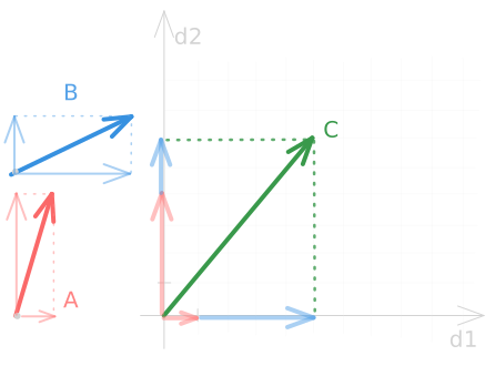
Under this constraint, matrix addition and subtraction can be understood intuitively as adding or subtracting the row vectors or column vectors one by one. Here we use the column-vector viewpoint as an example:

$$\mathbf{C}= \mathbf{A}+\mathbf{B}= \begin{bmatrix} {\color{#ff8383}1}\\ {\color{#ff8383}4} \end{bmatrix}+ \begin{bmatrix} {\color{#56a2e8}4}\\ {\color{#56a2e8}2} \end{bmatrix}= \begin{bmatrix} {\color{#39994b}5}\\ {\color{#39994b}6} \end{bmatrix}$$

Matrix addition as vector addition

Matrix Multiplication

If two matrices $\mathbf{A}\in \mathbb{R}^{n_1\times m_1}$ and $\mathbf{B}\in \mathbb{R}^{n_2\times m_2}$ are multiplied, then the prerequisite is $m1=n2$, that is, the number of columns of A = the number of rows of B.

Why is that? Let us start from the geometric intuition given by the row and column viewpoints.

The Linear-Transformation Viewpoint

Linear Projection of Column Vectors

Suppose three $2\times2$ matrices are each multiplied by the same $2\times1$ matrix $\mathbf{R}$:

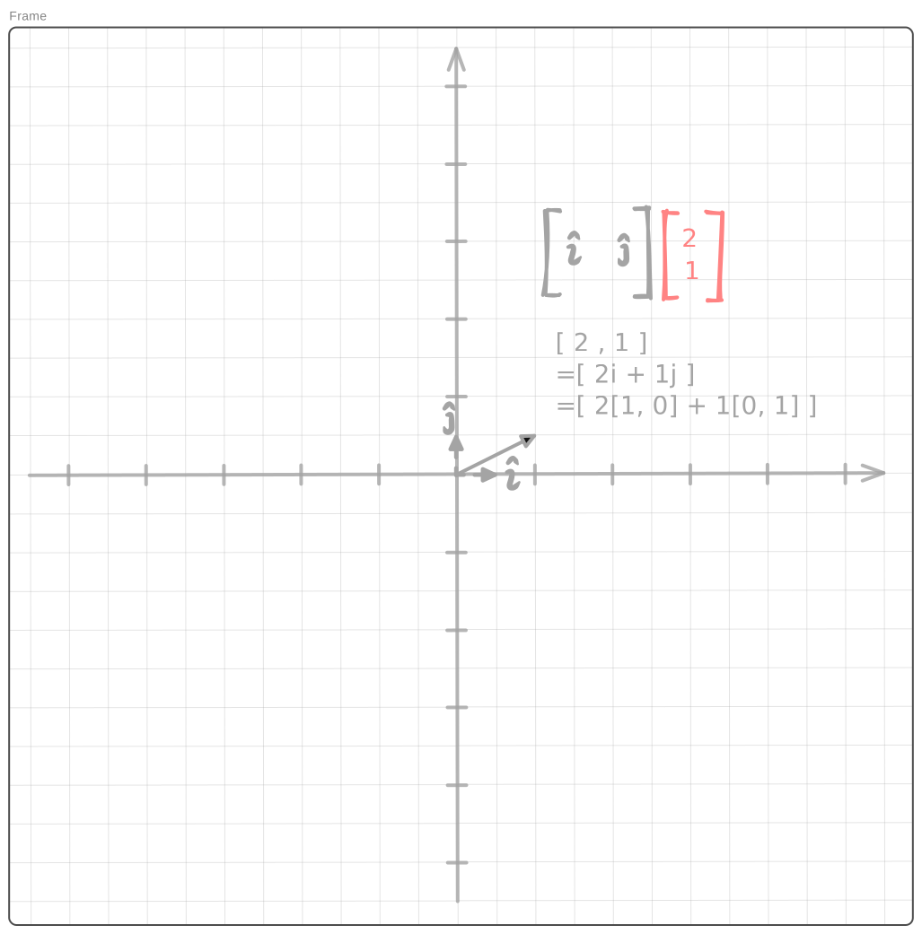
First, consider ${\color{#a4a4a4}\mathbf{N}}$ and ${\color{#ff8383}\mathbf{R}}$: $${\color{#a4a4a4}\mathbf{N}}{\color{#ff8383}\mathbf{R}}= {\color{#a4a4a4} \begin{bmatrix} 1 & 0\\ 0 & 1 \end{bmatrix}} {\color{#ff8383} \begin{bmatrix} 2\\ 1 \end{bmatrix}}= \begin{bmatrix} 2\\ 1 \end{bmatrix}\\$$

I deliberately colored the matrix ${\color{#a4a4a4}\mathbf{N}}$ in nickel gray, and of course that is intentional. Now look at the geometric picture of this operation:

Linear transformation N

The figure shows a standard two-dimensional Cartesian coordinate system, which lives in a ${\color{#a4a4a4}\text{gray}}$ two-dimensional linear space. Within that space, the only column vector of the matrix ${\color{#ff8383}\mathbf{R}}$, namely ${\color{#ff8383}\begin{bmatrix}2\\1\end{bmatrix}}$, lands at the point $(2, 1)$ on the axes.

Isn't that obvious? The vector $(2, 1)$ should of course land at position $(2, 1)$.

No—the heart of the intuition is hidden right there. If we want a vector to be placed perfectly in a two-dimensional Cartesian coordinate system, the following conditions are required:

• The vector must be two-dimensional, i.e. $(x1, y1)$
• Its form must be turned from $(x1, y1)$ into $(x1·\hat{i}, y1·\hat{j})$

Here, $\hat{i}, \hat{j}$ are the basis of the two-dimensional spanning space. Since we are currently focusing on vectors, we may call them basis vectors.

What the figure tells us is that the ${\color{#a4a4a4}\text{gray}}$ two-dimensional linear space, the matrix ${\color{#a4a4a4}\mathbf{N}}$, and the matrix ${\color{#ff8383}\mathbf{R}}$ are related in the following way:

• The vector basis ${\color{#a4a4a4}\hat{i}, \hat{j}}$ is exactly the two column vectors of the matrix ${\color{#a4a4a4}\mathbf{N}}$, namely ${\color{#a4a4a4}\begin{bmatrix}0\\1\end{bmatrix},\begin{bmatrix}0\\1\end{bmatrix}}$, and the number of basis vectors equals the dimension of the column vector of ${\color{#ff8383}\mathbf{R}}$, which is also the number of matrix rows.

This is the core intuition from the column viewpoint:

• The columns of matrix ${\color{#a4a4a4}\mathbf{N}}$ serve as the basis of the space and span a linear space
• The column vectors of matrix ${\color{#ff8383}\mathbf{R}}$ each fall into that linear space (column-vector dimension = the number of basis vectors in the space)

From a geometric viewpoint, this matrix product represents the result of a linear mapping of the column-vector family of matrix ${\color{#ff8383}\mathbf{R}}$ into the space defined by matrix ${\color{#a4a4a4}\mathbf{N}}$. In other words, the matrix ${\color{#ff8383}\mathbf{R}}$ undergoes the linear transformation defined by matrix ${\color{#a4a4a4}\mathbf{N}}$.

Matrix ${\color{#a4a4a4}\mathbf{N}}$ is a special linear transformation. Its basis vectors ${\color{#a4a4a4}\hat{i}, \hat{j}}$ are exactly the unit vectors themselves, so any matrix whose column vectors have dimension 2 is mapped to itself under this transformation. That is why it has a special name—the identity matrix—and the linear transformation it defines is called the identity transformation.

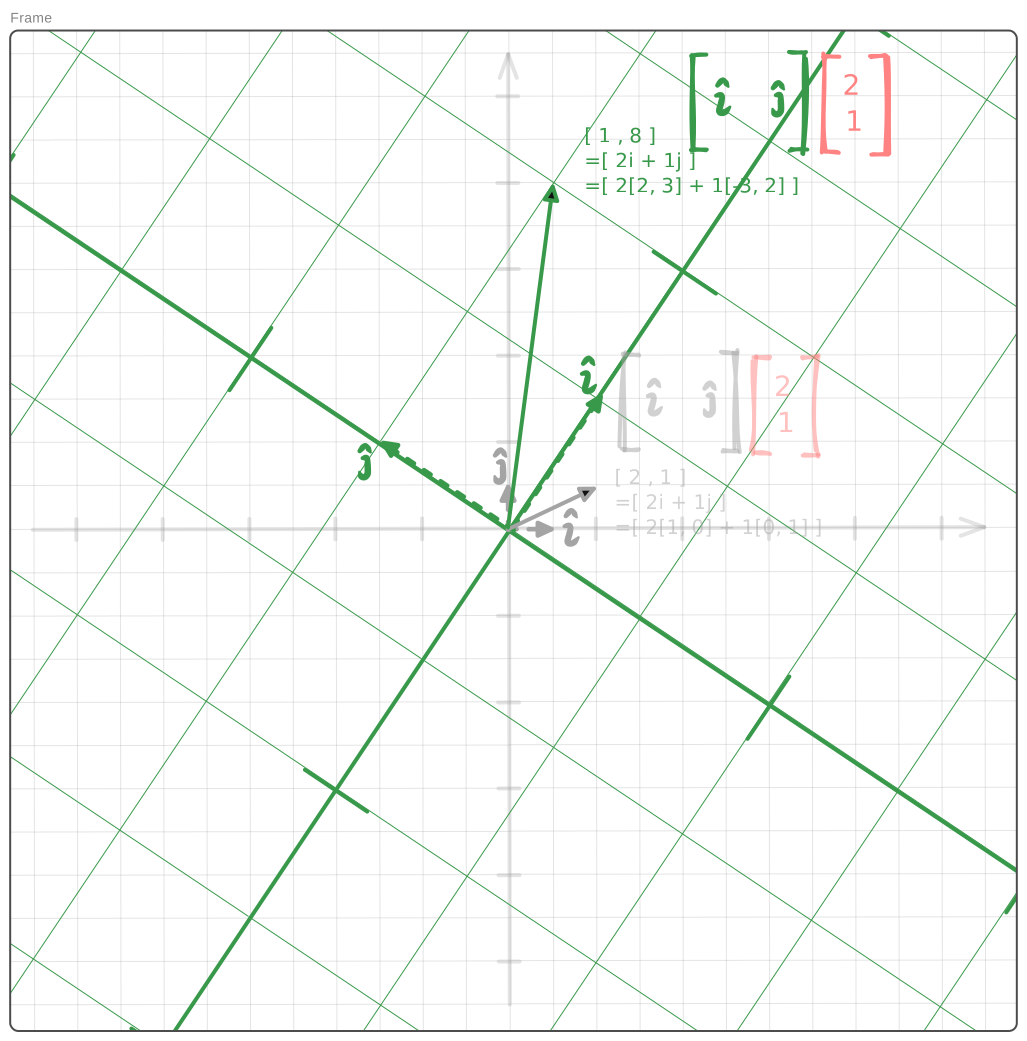
Let us look at a few more examples: $${\color{#39994b}\mathbf{G}}{\color{#ff8383}\mathbf{R}}= {\color{#39994b} \begin{bmatrix} 2 & -3\\ 3 & 2 \end{bmatrix}} {\color{#ff8383} \begin{bmatrix} 2\\ 1 \end{bmatrix}}= \begin{bmatrix} 1\\ 8 \end{bmatrix}\\$$

Linear transformation G

As shown, the basis vectors of matrix ${\color{#39994b}\mathbf{G}}$ are ${\color{#39994b}\hat{i}, \hat{j}}$. This pair of basis vectors can be projected into N-space by left-multiplying the identity matrix (identity transformation):

• mathematically, ${\color{#a4a4a4}\mathbf{N}}{\color{#39994b}\mathbf{G}}={\color{#39994b}\mathbf{G}}$,
• the projected basis vectors are ${\color{#39994b}\hat{i}=\begin{bmatrix}2\\3\end{bmatrix},\hat{j}=\begin{bmatrix}-3\\2\end{bmatrix}}$,
• visually, the linear transformation ${\color{#39994b}\mathbf{G}}$ rotates the original space basis counterclockwise by about $60°$, while also enlarging it by a factor a little greater than 3.

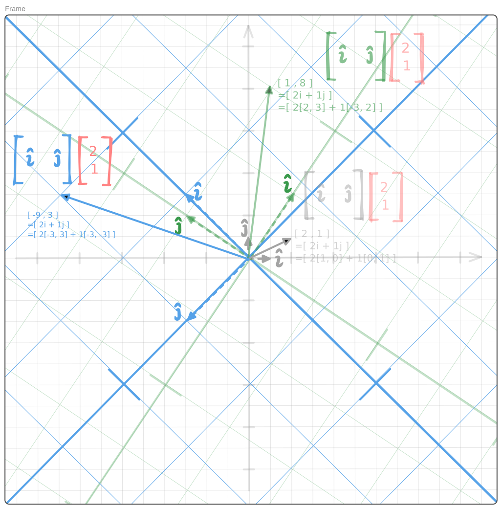
Now look at another one: $${\color{#56a2e8}\mathbf{B}}{\color{#ff8383}\mathbf{R}}= {\color{#56a2e8} \begin{bmatrix} -3 & -3\\ 3 & -3 \end{bmatrix}} {\color{#ff8383} \begin{bmatrix} 2\\ 1 \end{bmatrix}}= \begin{bmatrix} -9\\ 3 \end{bmatrix}$$

Linear transformation B

The geometric intuition is quite clear:

• the projected basis vectors are ${\color{#56a2e8}\hat{i}=\begin{bmatrix}-3\\3\end{bmatrix},\hat{j}=\begin{bmatrix}-3\\-3\end{bmatrix}}$,
• visually, the linear transformation ${\color{#56a2e8}\mathbf{N}}$ rotates the unit-space basis counterclockwise by $135°$, while also enlarging it by a factor slightly greater than 4.

Now we have the pattern.
These two-dimensional matrices can be understood geometrically in terms of rotation and scaling. They look a bit like a sheet of paper in front of you, whose appearance changes as your view tilts or zooms. And in fact, that is not far from the truth. Besides rotation and scaling, there are other possibilities as well. Imagine that a sheet of paper suddenly turns into a line in front of you—what two-dimensional matrix would correspond to that? You can work it out on your own.

Let us return to matrix multiplication. In the previous examples, $${\color{#a4a4a4}\mathbf{N}}{\color{#ff8383}\mathbf{R}}\\ {\color{#39994b}\mathbf{G}}{\color{#ff8383}\mathbf{R}}\\ {\color{#56a2e8}\mathbf{B}}{\color{#ff8383}\mathbf{R}}$$ we find that linear transformations of column vectors do have an order. For matrix $\mathbf{A}$ multiplied by $\mathbf{B}$:

• in formula form, we write $\mathbf{A}\mathbf{B}$,
• intuitively, it means that the linear transformation defined by the matrix on the left, $\mathbf{A}$, acts on the column vectors inside the matrix on the right, $\mathbf{B}$.

We can also understand it in function form, which makes the formula feel more natural: $${\color{#a4a4a4}\mathbf{n}}({\color{#ff8383}\mathbf{R}})\\ {\color{#39994b}\mathbf{g}}({\color{#a4a4a4}\mathbf{n}}({\color{#ff8383}\mathbf{R}}))\\ {\color{#56a2e8}\mathbf{b}}({\color{#a4a4a4}\mathbf{n}}({\color{#ff8383}\mathbf{R}}))$$

Now, with this geometric intuition for linear transformations in mind, let us think about a question.
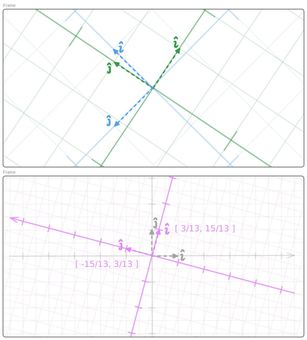
Suppose the linear-transformation effect of ${\color{#56a2e8}\mathbf{B}}$ is actually a composition of several different matrix transformations, for example: $$\begin{aligned} {\color{#56a2e8}\mathbf{B}} &={\color{#e28ef8}\mathbf{P}}{\color{#39994b}\mathbf{G}} \\ {\color{#56a2e8} \begin{bmatrix} -3 & -3\\ 3 & -3 \end{bmatrix}} &={\color{#e28ef8} \begin{bmatrix} \hat{i} & \hat{j} \end{bmatrix}} {\color{#39994b} \begin{bmatrix} 2 & -3\\ 3 & 2 \end{bmatrix}} \end{aligned}$$

Can you picture the geometric intuition of the linear transformation ${\color{#e28ef8}\mathbf{P}}$?
The result is shown in Appendix - Linear Transformation P.

Linear Projection of Row Vectors

If you are comfortable with the column-vector view of linear transformations above, then the row-vector case is easy to understand.

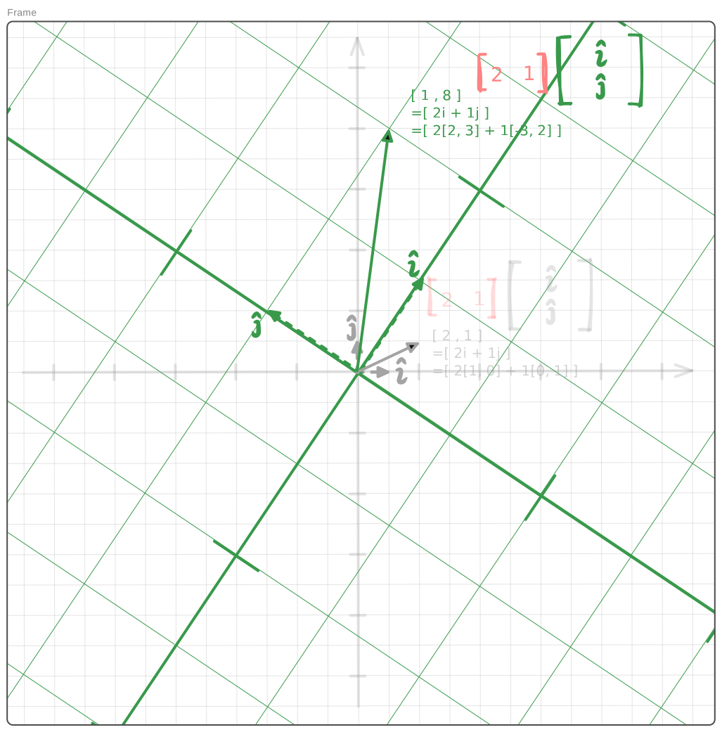
Please look at the linear transformation shown below:

Linear transformation G — row-vector viewpoint

At first glance, it looks exactly like the previous linear transformation ${\color{#39994b}\mathbf{G}}$.

Exactly. But the difference is that the geometric picture here represents the linear transformation ${\color{#39994b}\mathbf{G^T}}$, and the matrix product involved is: $$\begin{aligned} {\color{#ff8383}\mathbf{R^T}}{\color{#39994b}\mathbf{G^T}}&= {\color{#ff8383} \begin{bmatrix} 2 & 1 \end{bmatrix}} {\color{#39994b} \begin{bmatrix} 2 & 3\\ -3 & 2 \end{bmatrix}}&= {\color{#ff8383} \begin{bmatrix} 2 & 1 \end{bmatrix}} {\color{#39994b} \begin{bmatrix} \hat{i}\\ \hat{j} \end{bmatrix}}&= \begin{bmatrix} 1 & 8\\ \end{bmatrix} \end{aligned}$$

Compare this with what we said earlier from the column-vector viewpoint:

Linear transformations of column vectors do have an order. For matrix $\mathbf{A}$ multiplied by $\mathbf{B}$:

• in formula form, we write $\mathbf{A}\mathbf{B}$,
• intuitively, it means that the linear transformation defined by the matrix on the left, $\mathbf{A}$, acts on the column vectors inside the matrix on the right, $\mathbf{B}$.

In the same style, the row-vector viewpoint follows this rule:

Linear transformations of row vectors also have an order. For matrix $\mathbf{A}$ multiplied by $\mathbf{B}$:

• in formula form, we write $\mathbf{A}\mathbf{B}$,
• intuitively, it means that the linear transformation defined by the matrix on the right, $\mathbf{B}$, acts on the row vectors inside the matrix on the left, $\mathbf{A}$.

From the column-vector linear-projection viewpoint, matrix multiplication is ${\color{#39994b}\mathbf{G}}{\color{#ff8383}\mathbf{R}}$.
From the row-vector linear-projection viewpoint, matrix multiplication is ${\color{#ff8383}\mathbf{R^T}}{\color{#39994b}\mathbf{G^T}}$.

In our example, their geometric intuition is the same:
the vectors inside the same matrix ${\color{#ff8383}\mathbf{R}}$ are projected into the same linear space spanned by the same set of basis vectors ${\color{#39994b}\hat{i},\hat{j}}$.

The Inner-Product (Dot-Product / Scalar-Product) Viewpoint — Row × Column

Let the left matrix be $\mathbf{A}\in\mathbb{R}^{m\times n}$ and the right matrix be $\mathbf{B}\in\mathbb{R}^{n\times p}$.
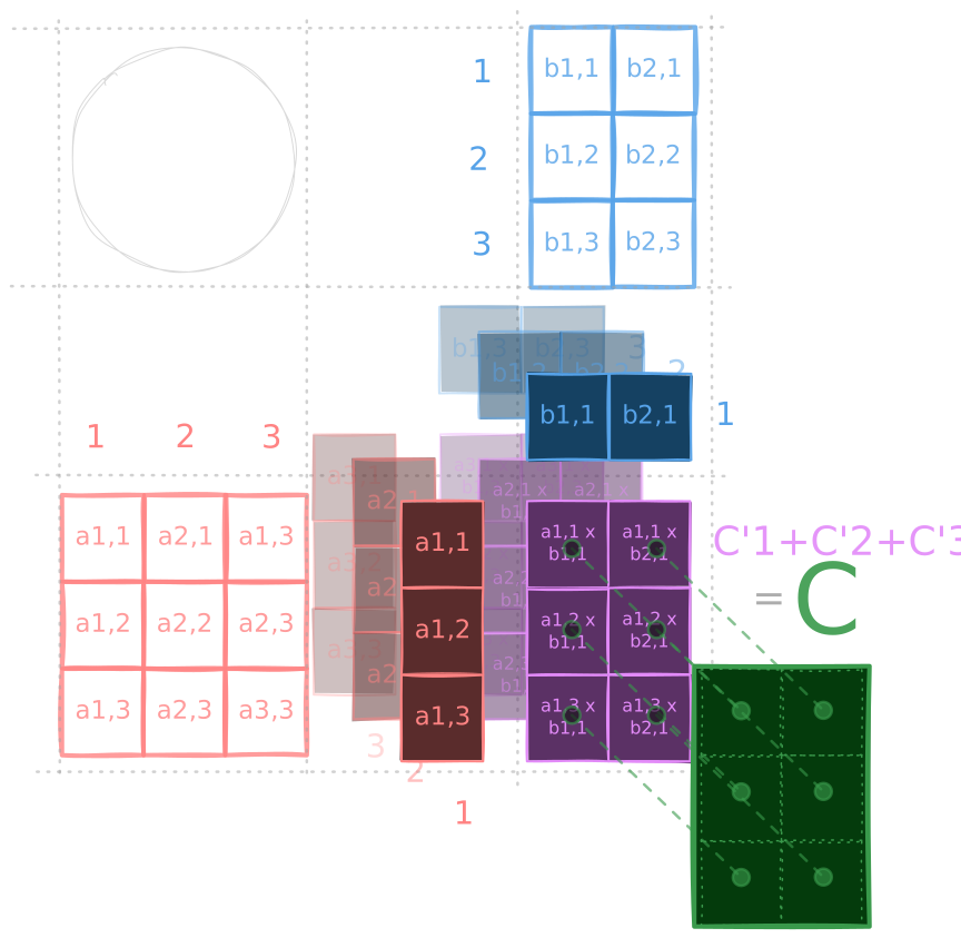
The matrix-multiplication formula is: $$\begin{aligned} \mathbf{C}=\mathbf{A}\mathbf{B} &= \begin{bmatrix} a_{11} & a_{12} & \cdots & a_{1n}\\ a_{21} & a_{22} & \cdots & a_{2n}\\ \vdots & \vdots & \ddots & \vdots\\ a_{m1} & a_{m2} & \cdots & a_{mn} \end{bmatrix} \begin{bmatrix} b_{11} & b_{12} & \cdots & b_{1p}\\ b_{21} & b_{22} & \cdots & b_{2p}\\ \vdots & \vdots & \ddots & \vdots\\ b_{n1} & b_{n2} & \cdots & b_{np} \end{bmatrix} \\[1em] &= \begin{bmatrix} \mathbf{a}_1^\mathsf{T}\\ \mathbf{a}_2^\mathsf{T}\\ \vdots\\ \mathbf{a}_m^\mathsf{T} \end{bmatrix} \begin{bmatrix} \mathbf{b}_1 & \mathbf{b}_2 & \cdots & \mathbf{b}_p \end{bmatrix} \\[1em] &= \begin{bmatrix} \mathbf{a}_1^\mathsf{T}\mathbf{b}_1 & \mathbf{a}_1^\mathsf{T}\mathbf{b}_2 & \cdots & \mathbf{a}_1^\mathsf{T}\mathbf{b}_p\\ \mathbf{a}_2^\mathsf{T}\mathbf{b}_1 & \mathbf{a}_2^\mathsf{T}\mathbf{b}_2 & \cdots & \mathbf{a}_2^\mathsf{T}\mathbf{b}_p\\ \vdots & \vdots & \ddots & \vdots\\ \mathbf{a}_m^\mathsf{T}\mathbf{b}_1 & \mathbf{a}_m^\mathsf{T}\mathbf{b}_2 & \cdots & \mathbf{a}_m^\mathsf{T}\mathbf{b}_p \end{bmatrix} \\[1em] &= \begin{bmatrix} c_{11} & c_{12} & \cdots & c_{1p}\\ c_{21} & c_{22} & \cdots & c_{2p}\\ \vdots & \vdots & \ddots & \vdots\\ c_{m1} & c_{m2} & \cdots & c_{mp} \end{bmatrix}, \end{aligned}$$

Here, the $i$-th row vector of $\mathbf{A}$ is denoted by $\mathbf{a}_i^\mathsf{T}\in\mathbb{R}^{1\times n}$, and the $j$-th column vector of $\mathbf{B}$ is denoted by $\mathbf{b}_j\in\mathbb{R}^{n\times 1}$.

The element in the $i$-th row and $j$-th column of the resulting matrix $\mathbf{C}$ is denoted by $\mathbf{c}_{ij}$, and it represents the dot product between the row vector $\mathbf{a}_i^\mathsf{T}$ from the left matrix and the column vector $\mathbf{b}_j$ from the right matrix: $$c_{ij}= \mathbf{a}_i^\mathsf{T}\mathbf{b}_j= \sum_{k=1}^{n}a_{ik}b_{kj}$$

Let us build the intuition step by step through an example: $$\begin{aligned} \mathbf{C}={\color{#ff8383}\mathbf{A}}{\color{#56a2e8}\mathbf{B}} &= {\color{#ff8383} \begin{bmatrix} 3 & 2 & 1\\ 6 & 4 & 2\\ 1 & 2 & 5 \end{bmatrix}} {\color{#56a2e8} \begin{bmatrix} 1 & 2\\ 3 & 1\\ 0 & 4 \end{bmatrix}} \\ &= {\color{#ff8383} \begin{bmatrix} \mathbf{a}_1^\mathsf{T}\\ \mathbf{a}_2^\mathsf{T}\\ \mathbf{a}_3^\mathsf{T} \end{bmatrix}} {\color{#56a2e8} \begin{bmatrix} \mathbf{b}_1 & \mathbf{b}_2 \end{bmatrix}} \\ &= \begin{bmatrix} {\color{#ff8383}\mathbf{a}_1^\mathsf{T}}{\color{#56a2e8}\mathbf{b}_1} & {\color{#ff8383}\mathbf{a}_1^\mathsf{T}}{\color{#56a2e8}\mathbf{b}_2}\\ {\color{#ff8383}\mathbf{a}_2^\mathsf{T}}{\color{#56a2e8}\mathbf{b}_1} & {\color{#ff8383}\mathbf{a}_2^\mathsf{T}}{\color{#56a2e8}\mathbf{b}_2}\\ {\color{#ff8383}\mathbf{a}_3^\mathsf{T}}{\color{#56a2e8}\mathbf{b}_1} & {\color{#ff8383}\mathbf{a}_3^\mathsf{T}}{\color{#56a2e8}\mathbf{b}_2} \end{bmatrix} =\begin{bmatrix} {\color{#ff8383}\mathbf{a}_1}\cdot{\color{#56a2e8}\mathbf{b}_1} & {\color{#ff8383}\mathbf{a}_1}\cdot{\color{#56a2e8}\mathbf{b}_2}\\ {\color{#ff8383}\mathbf{a}_2}\cdot{\color{#56a2e8}\mathbf{b}_1} & {\color{#ff8383}\mathbf{a}_2}\cdot{\color{#56a2e8}\mathbf{b}_2}\\ {\color{#ff8383}\mathbf{a}_3}\cdot{\color{#56a2e8}\mathbf{b}_1} & {\color{#ff8383}\mathbf{a}_3}\cdot{\color{#56a2e8}\mathbf{b}_2} \end{bmatrix}\\ &= \begin{bmatrix} 9 & 12\\ 18 & 24\\ 7 & 24 \end{bmatrix} \end{aligned}$$

Here, if we take any one of these dot products, say ${\color{#ff8383}q} \cdot {\color{#56a2e8}k} = {\color{#ff8383}a_i} \cdot {\color{#56a2e8}b_j}$, its expanded formula is: $${\color{#ff8383}\mathbf{q}}\cdot{\color{#56a2e8}\mathbf{k}}= {\color{#ff8383} \begin{bmatrix} q_1 & q_2 & q_3 \end{bmatrix}} {\color{#56a2e8} \begin{bmatrix} k_1 \\ k_2 \\ k_3 \end{bmatrix}}= \begin{bmatrix} {\color{#ff8383}q_1}{\color{#56a2e8}k_1} + {\color{#ff8383}q_2}{\color{#56a2e8}k_2} + {\color{#ff8383}q_3}{\color{#56a2e8}k_3} \end{bmatrix}$$

The geometric intuition of this computation process is shown here:

Row-column dot product

It looks like a network structure, in which:

• the red row vectors (objects) form the nodes on the left,
• the blue column vectors (operators) form the connecting edges,
• the green row vectors (dot-product results) form the output nodes on the right.

The result of taking the dot product between a row vector from the left matrix and a column vector from the right matrix, $a_i^Tb_j=a_i \cdot b_j$, is a scalar value (it is not represented as a $1\times1$ matrix in the matrix result).

Besides being understood as the green nodes in the network above, this scalar also has a more general geometric interpretation.

Intuition for the Vector Dot Product

The dot product of two vectors, ${\color{#ff8383}q} \cdot {\color{#56a2e8}k}$ (I secretly reduced the dimension a bit for the sake of the following demonstration), actually has a hidden equality: $$\begin{aligned} {\color{#ff8383}\mathbf{q}}\cdot{\color{#56a2e8}\mathbf{k}}= {\color{#ff8383}(q_1 , q_2)\cdot} {\color{#56a2e8}(k_1, k_2)} &= {\color{#ff8383}q_1}{\color{#56a2e8}k_1}+ {\color{#ff8383}q_2}{\color{#56a2e8}k_2}\\ &= \begin{bmatrix} {\color{#ff8383}q_1}{\color{#56a2e8}k_1} + {\color{#ff8383}q_2}{\color{#56a2e8}k_2} \end{bmatrix}\\ &= {\color{#ff8383} \begin{bmatrix} q_1 \\ q_2 \end{bmatrix}} \cdot {\color{#56a2e8} \begin{bmatrix} k_1 \\ k_2 \end{bmatrix}}\\ &= {\color{#ff8383} \begin{bmatrix} q_1 & q_2 \end{bmatrix}} {\color{#56a2e8} \begin{bmatrix} k_1 \\ k_2 \end{bmatrix}}\\ &= {\color{#56a2e8} \begin{bmatrix} k_1 & k_2 \end{bmatrix}} {\color{#ff8383} \begin{bmatrix} q_1 \\ q_2 \end{bmatrix}} \end{aligned}$$

From the linear-transformation viewpoint above, as long as we can grasp $\hat{i},\hat{j}$, the operation in this equality is easy to understand: one vector defines a linear space that acts on the other vector. This leaves us with the question: when the dimension of $\hat{i},\hat{j}$ is 1, how should we form a geometric intuition for the linear space they define?

Let us plug some numbers into the expression: $${\color{#ff8383}\mathbf{q}}\cdot{\color{#a4a4a4}\mathbf{k}}= {\color{#ff8383} \begin{bmatrix} 3 & 2 \end{bmatrix}} {\color{#a4a4a4} \begin{bmatrix} x \\ y \end{bmatrix}}$$

Now, with $\color{#ff8383}\hat{i}=[3], \hat{j}=[2]$, what is the linear space defined by them? The derivation goes as follows:

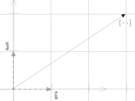
First, in the linear space of unit vectors, the vector $q=(3, 2)$ is projected into it.

Vector $(3, 2)$

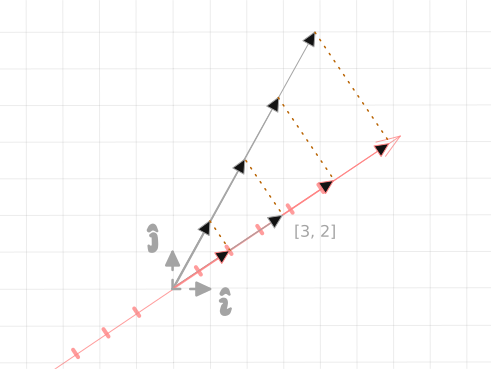
Next, place a unit number line (with unit length 1) so that its positive direction aligns with the vector $q=(3, 2)$. Other vectors can then be orthogonally projected onto this number line to obtain a new representation, and this process satisfies:

1. Vector addition in the unit space still holds after projection onto the number line (additivity)
2. Vectors in the unit space with the same direction but different lengths still preserve the same proportion after projection onto the number line (homogeneity)

Orthogonal projection of vectors onto a number line

Conjecture: after vector $k$ undergoes the linear transformation defined by the one-dimensional matrix $\begin{bmatrix}3 & 2\end{bmatrix}$, the result can be understood geometrically as the length of the orthogonal projection of the vector onto the number line.

If this is true, then under the space defined by the identity matrix, we should have:

• the result of $\begin{bmatrix} 3 & 2 \end{bmatrix}\begin{bmatrix}a \\ b \end{bmatrix}$ equals the projection length of $(a, b)$

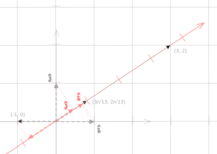
Some projection cases are shown below: Projection cases for several vectors

• the signed projection length of $(1, 0)$ is $3/\sqrt{13}$, while
  $$\begin{bmatrix}3 & 2\end{bmatrix}\begin{bmatrix}1 \\ 0\end{bmatrix} =(3, 2)\cdot(1, 0)=3\cdot1 + 2\cdot0 =3 = \sqrt{13} \cdot 3/\sqrt{13}$$

• the signed projection length of $(-1, 0)$ is $-3/\sqrt{13}$, while
  $$\begin{bmatrix}3 & 2\end{bmatrix}\begin{bmatrix}-1 \\ 0\end{bmatrix} =(3, 2)\cdot(-1, 0)=3\cdot(-1) + 2\cdot0 =-3 = -\sqrt{13} \cdot 3/\sqrt{13}$$

• the signed projection length of $(0, 1)$ is $2/\sqrt{13}$, while
  $$\begin{bmatrix}3 & 2\end{bmatrix}\begin{bmatrix}0 \\ 1\end{bmatrix} =(3, 2)\cdot(0, 1)=3\cdot0 + 2\cdot1 =2 = \sqrt{13} \cdot 2/\sqrt{13}$$

• the signed projection length of $(3, 2)$ is $\sqrt{13}$, while
  $$\begin{bmatrix}3 & 2\end{bmatrix}\begin{bmatrix}3 \\ 2\end{bmatrix} =(3, 2)\cdot(3, 2)=3\cdot3 + 2\cdot2 = 13 = \sqrt{13} \cdot \sqrt{13}$$

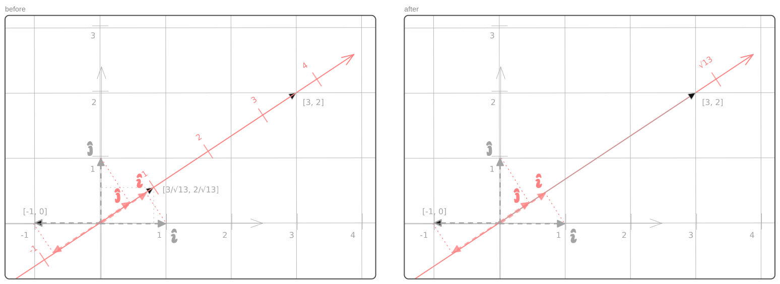
So the conjecture does not hold. But strikingly, we find that the discrepancy lies in $\sqrt{13}$ and $-\sqrt{13}$. Then suppose the unit length on our number line is not $1$ but $\sqrt{13}$, as shown below:

Changing the unit length on the number line

Now it matches: $$\begin{aligned} \begin{bmatrix}3 & 2\end{bmatrix}\begin{bmatrix}3 \\ 2\end{bmatrix} &=(3, 2)\cdot(3, 2)\\ &=3\cdot3 + 2\cdot2 = 13\\ &= \sqrt{13} \cdot \sqrt{13}\\ &= reading on the scale of the number line in the direction where the orthogonal projection lies \times orthogonal projection length \end{aligned}$$

Therefore, after vector $k$ undergoes the linear transformation defined by the one-dimensional matrix $\begin{bmatrix}3 & 2\end{bmatrix}$, the result can be understood geometrically as:
the orthogonal projection length of vector $k$ onto a number line whose unit length equals that of vector $(3, 2)$, multiplied by the scale reading at the point where the projection lands.

Then which one-dimensional matrix corresponds to the number line in the figure on the left? You can work that out on your own.

This proof refers to the mathematics creator 3Blue1Brown's Linear Algebra: Dot Products. His linear algebra series is very much worth watching.

With the geometric intuition of vector dot products in place, matrix operations become even more vivid from the dot-product viewpoint.

The Outer-Product Viewpoint — Column × Row

Let the $k$-th column vector of $\mathbf{A}$ be denoted by $\mathbf{a}_k\in\mathbb{R}^{m\times 1}$, and the $k$-th row vector of $\mathbf{B}$ be denoted by $\mathbf{b}_k^\mathsf{T}\in\mathbb{R}^{1\times p}$. Then the formula from the outer-product viewpoint is:

$$\begin{aligned} \mathbf{C}=\mathbf{A}\mathbf{B} &=\begin{bmatrix} a_{11} & a_{12} & \cdots & a_{1n}\\ a_{21} & a_{22} & \cdots & a_{2n}\\ \vdots & \vdots & \ddots & \vdots\\ a_{m1} & a_{m2} & \cdots & a_{mn} \end{bmatrix} \begin{bmatrix} b_{11} & b_{12} & \cdots & b_{1p}\\ b_{21} & b_{22} & \cdots & b_{2p}\\ \vdots & \vdots & \ddots & \vdots\\ b_{n1} & b_{n2} & \cdots & b_{np} \end{bmatrix}\\ &=\begin{bmatrix} \mathbf{a}_1 & \mathbf{a}_2 & \cdots & \mathbf{a}_n \end{bmatrix} \begin{bmatrix} \mathbf{b}_1^\mathsf{T}\\ \mathbf{b}_2^\mathsf{T}\\ \vdots\\ \mathbf{b}_n^\mathsf{T} \end{bmatrix}\\ &=\mathbf{a}_1\mathbf{b}_1^\mathsf{T} + \mathbf{a}_2\mathbf{b}_2^\mathsf{T} + \cdots + \mathbf{a}_n\mathbf{b}_n^\mathsf{T} =\mathbf{a}_1\otimes\mathbf{b}_1 + \mathbf{a}_2\otimes\mathbf{b}_2 + \cdots + \mathbf{a}_n\otimes\mathbf{b}_n\\ &=\begin{bmatrix} a_{11}\\ a_{21}\\ \vdots\\ a_{m1} \end{bmatrix} \begin{bmatrix} b_{11} & b_{12} & \cdots & b_{1p} \end{bmatrix} + \begin{bmatrix} a_{12}\\ a_{22}\\ \vdots\\ a_{m2} \end{bmatrix} \begin{bmatrix} b_{21} & b_{22} & \cdots & b_{2p} \end{bmatrix} + \cdots + \begin{bmatrix} a_{1n}\\ a_{2n}\\ \vdots\\ a_{mn} \end{bmatrix} \begin{bmatrix} b_{n1} & b_{n2} & \cdots & b_{np} \end{bmatrix}\\ &= \begin{bmatrix} a_{11}b_{11} & a_{11}b_{12} & \cdots & a_{11}b_{1p}\\ a_{21}b_{11} & a_{21}b_{12} & \cdots & a_{21}b_{1p}\\ \vdots & \vdots & \ddots & \vdots\\ a_{m1}b_{11} & a_{m1}b_{12} & \cdots & a_{m1}b_{1p} \end{bmatrix} + \begin{bmatrix} a_{12}b_{21} & a_{12}b_{22} & \cdots & a_{12}b_{2p}\\ a_{22}b_{21} & a_{22}b_{22} & \cdots & a_{22}b_{2p}\\ \vdots & \vdots & \ddots & \vdots\\ a_{m2}b_{21} & a_{m2}b_{22} & \cdots & a_{m2}b_{2p} \end{bmatrix} + \cdots + \begin{bmatrix} a_{1n}b_{n1} & a_{1n}b_{n2} & \cdots & a_{1n}b_{np}\\ a_{2n}b_{n1} & a_{2n}b_{n2} & \cdots & a_{2n}b_{np}\\ \vdots & \vdots & \ddots & \vdots\\ a_{mn}b_{n1} & a_{mn}b_{n2} & \cdots & a_{mn}b_{np} \end{bmatrix}\\ &=\sum_{k=1}^{n}\mathbf{a}_k\mathbf{b}_k^\mathsf{T} \end{aligned}$$

We still use the example from the inner-product viewpoint: $$\begin{aligned} \mathbf{C}={\color{#ff8383}\mathbf{A}}{\color{#56a2e8}\mathbf{B}} &={\color{#ff8383} \begin{bmatrix} 3 & 2 & 1\\ 6 & 4 & 2\\ 1 & 2 & 5 \end{bmatrix}} {\color{#56a2e8} \begin{bmatrix} 1 & 2\\ 3 & 1\\ 0 & 4 \end{bmatrix}}\\ &={\color{#ff8383} \begin{bmatrix} \mathbf{a}_1 & \mathbf{a}_2 & \mathbf{a}_3 \end{bmatrix}} {\color{#56a2e8} \begin{bmatrix} \mathbf{b}_1^\mathsf{T}\\ \mathbf{b}_2^\mathsf{T}\\ \mathbf{b}_3^\mathsf{T} \end{bmatrix}}\\ &={\color{#ff8383}\mathbf{a}_1}{\color{#56a2e8}\mathbf{b}_1^\mathsf{T}}+ {\color{#ff838380}\mathbf{a}_2}{\color{#56a2e880}\mathbf{b}_2^\mathsf{T}}+ {\color{#ff838350}\mathbf{a}_3}{\color{#56a2e850}\mathbf{b}_3^\mathsf{T}}= {\color{#ff8383}\mathbf{a}_1}\otimes{\color{#56a2e8}\mathbf{b}_1}+ {\color{#ff838380}\mathbf{a}_2}\otimes{\color{#56a2e880}\mathbf{b}_2}+ {\color{#ff838350}\mathbf{a}_3}\otimes{\color{#56a2e850}\mathbf{b}_3}\\ &={\color{#ff8383} \begin{bmatrix} 3\\ 6\\ 1 \end{bmatrix}} {\color{#56a2e8} \begin{bmatrix} 1 & 2 \end{bmatrix}}+ {\color{#ff838380} \begin{bmatrix} 2\\ 4\\ 2 \end{bmatrix}} {\color{#56a2e880} \begin{bmatrix} 3 & 1 \end{bmatrix}}+ {\color{#ff838350} \begin{bmatrix} 1\\ 2\\ 5 \end{bmatrix}} {\color{#56a2e850} \begin{bmatrix} 0 & 4 \end{bmatrix}}\\ &=\begin{bmatrix} 3 & 6\\ 6 & 12\\ 1 & 2 \end{bmatrix}+ \begin{bmatrix} 6 & 2\\ 12 & 4\\ 6 & 2 \end{bmatrix}+ \begin{bmatrix} 0 & 4\\ 0 & 8\\ 0 & 20 \end{bmatrix}\\ &=\begin{bmatrix} 9 & 12\\ 18 & 24\\ 7 & 24 \end{bmatrix} \end{aligned}$$

Column-row outer product

The outer product between a column vector from the left matrix and a row vector from the right matrix, $a_i^Tb_j=a_i \otimes b_j$, appears as a submatrix, and the sum of all such submatrices equals the result matrix $C$. This is the geometric intuition from the outer-product viewpoint.

Closing Remarks

As a mathematical form, matrices do a remarkably good job of decomposing and analyzing how parts of physical reality operate.
Because of their power, more and more domains of knowledge treat matrices as an essential component. Without the necessary background, some of those fields can look like towering mountains, breathtaking in their scale.

And yet every mountain is built from countless tiny grains. Looked at from one angle it is a ridge, from another a peak. The right prerequisite knowledge provides the right viewpoint. Just like the linear space of a one-dimensional matrix, there is always a way to flatten the terrain, walk it as if on level ground, and one day look down from the summit.

This article offered geometric intuition for matrices from several common viewpoints, and I hope it helps.

Appendix

Linear Transformation P

Linear transformation P

Imagine the linear space of $\color{#56a2e8}\mathbf{B}$ as a blue sheet of paper,
while the linear space of ${\color{#39994b}\mathbf{G}}$ is a green sheet of paper.

The geometric intuition of ${\color{#e28ef8}\mathbf{P}}$ is therefore:
what must be done to turn the green sheet into the blue sheet?

Intuitively: rotate it counterclockwise by nearly $90°$, while also enlarging it by a factor a little greater than 1.